Working with fastai2 - Low-Level API
This notebook contains some experiments made with fastai's low level api with the MNIST dataset


These are the imports for everything we'll be using in this notebook
from torch import nn

from fastai.vision.all import *
from fastai.callback.hook import summary
from fastai.callback.schedule import fit_one_cycle, lr_find
from fastai.callback.progress import ProgressCallback

from fastai.data.core import Datasets, DataLoaders, show_at
from fastai.data.external import untar_data, URLs
from fastai.data.transforms import Categorize, GrandparentSplitter, parent_label, ToTensor, IntToFloatTensor, Normalize

from fastai.layers import Flatten
from fastai.learner import Learner

from fastai.metrics import accuracy, CrossEntropyLossFlat

from fastai.vision.augment import CropPad, RandomCrop, PadMode
from fastai.vision.core import PILImageBW
from fastai.vision.utils import get_image_files
import matplotlib.pyplot as plt
plt.style.use('dark_background')
grabbing our data
path = untar_data(URLs.MNIST)
items = get_image_files(path)
items[0]
im = PILImageBW.create(items[0]); im.show()

Split our data with GrandparentSplitter, which will make use of a train and valid folder.
splits = GrandparentSplitter(train_name='training', valid_name='testing')
splits = splits(items)
splits[0][:5], splits[1][:5]
-
Make a
Datasets -
Expects items, transforms for describing our problem, and a splitting method
dsrc = Datasets(items, tfms=[[PILImageBW.create], [parent_label, Categorize]],
                  splits = splits)
show_at(dsrc.train, 3)

Next we need to give ourselves some transforms on the data! These will need to:
- Ensure our images are all the same size
- Make sure our output are the
tensorour models are wanting - Give some image augmentation
tfms = [ToTensor(), CropPad(size=34, pad_mode=PadMode.Zeros), RandomCrop(size=28)]
-
ToTensor: Converts to tensor -
CropPadandRandomCrop: Resizing transforms - Applied on the
CPUviaafter_item
gpu_tfms = [IntToFloatTensor(), Normalize()]
-
IntToFloatTensor: Converts to a float -
Normalize: Normalizes data
dls = dsrc.dataloaders(bs=128, after_item=tfms, after_batch=gpu_tfms)
dls.show_batch()

xb, yb = dls.one_batch()
xb.shape, yb.shape
dls.c
So our input shape will be a [128 x 1 x 28 x 28] and our output shape will be a [128] tensor that we need to condense into 10 classes
def conv(ni, nf): return nn.Conv2d(ni, nf, kernel_size=3, stride=2, padding=1)
Here we can see our ni is equivalent to the depth of the filter, and nf is equivalent to how many filters we will be using. (Fun fact this always has to be divisible by the size of our image).
Batch Normalization
As we send our tensors through our model, it is important to normalize our data throughout the network. Doing so can allow for a much larger improvement in training speed, along with allowing each layer to learn independantly (as each layer is then re-normalized according to it's outputs)
def bn(nf): return nn.BatchNorm2d(nf)
nf will be the same as the filter output from our previous convolutional layer
Activation functions
They give our models non-linearity and work with the weights we mentioned earlier along with a bias through a process called back-propagation. These allow our models to learn and perform more complex tasks because they can choose to fire or activate one of those neurons mentioned earlier. On a simple sense, let's look at the ReLU activation function. It operates by turning any negative values to zero, as visualized below:
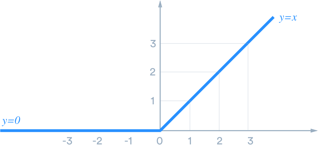
def ReLU(): return nn.ReLU(inplace=False)
model = nn.Sequential(
    conv(1, 8),
    bn(8),
    ReLU(),
    conv(8, 16),
    bn(16),
    ReLU(),
    conv(16,32),
    bn(32),
    ReLU(),
    conv(32, 16),
    bn(16),
    ReLU(),
    conv(16, 10),
    bn(10),
    Flatten()
)
learn = Learner(dls, model, loss_func=CrossEntropyLossFlat(), metrics=accuracy)
learn.summary()
learn.summary also tells us:
- Total parameters
- Trainable parameters
- Optimizer
- Loss function
- Applied
Callbacks
learn.lr_find()

learn.fit_one_cycle(3, lr_max=1e-1)
def conv2(ni, nf): return ConvLayer(ni, nf, stride=2)
net = nn.Sequential(
    conv2(1,8),
    conv2(8,16),
    conv2(16,32),
    conv2(32,16),
    conv2(16,10),
    Flatten()
)
learn = Learner(dls, net, loss_func=CrossEntropyLossFlat(), metrics=accuracy)
learn.fit_one_cycle(3, lr_max=1e-1)
class ResBlock(Module):

    def __init__(self, nf):
        self.conv1 = ConvLayer(nf, nf)
        self.conv2 = ConvLayer(nf, nf)


    def forward(self, x): return x + self.conv2(self.conv1(x))
- Class notation
__init__forward
net = nn.Sequential(
    conv2(1,8),
    ResBlock(8),
    conv2(8,16),
    ResBlock(16),
    conv2(16,32),
    ResBlock(32),
    conv2(32,16),
    ResBlock(16),
    conv2(16,10),
    Flatten()
)
Awesome! We're building a pretty substantial model here. Let's try to make it even simpler. We know we call a convolutional layer before each ResBlock and they all have the same filters, so let's make that layer!
def conv_and_res(ni, nf): return nn.Sequential(conv2(ni, nf), ResBlock(nf))
net = nn.Sequential(
    conv_and_res(1,8),
    conv_and_res(8,16),
    conv_and_res(16,32),
    conv_and_res(32,16),
    conv2(16,10),
    Flatten()
)
And now we have something that resembles a ResNet! Let's see how it performs
learn = Learner(dls, net, loss_func=CrossEntropyLossFlat(), metrics=accuracy)
learn.lr_find()

learn.fit_one_cycle(3, lr_max=1e-1)
learn.path = Path('')
learn.export(fname='export.pkl')